Last week I was lucky enough to have another paper come out, this time in BMC Bioinformatics:

“nRCFV: a new, dataset-size-independent metric to quantify compositional heterogeneity in nucleotide and amino acid datasets”

It’s a less elegant title than usual, I’ll admit! In addition, for a biological paper, there is an astounding lack of animals, plants, fungi, bacteria or archaea in it. So, what on earth does that title actually mean? And what is that dazzling equation in the header?

Compositional heterogeneity is the key word in the salad – and it is a big problem for many of our current phylogenetic models. Phylogeny is the study of the relationships between animals, as we try and work out their shared biological history and patterns of descent – a bit like building a family tree, but on a far larger scale. To do this, biologists collect DNA or amino acid (protein) sequences from the organisms they are interested in (called an alignment) and combine this information with mathematical models to construct trees of relationships. However, these models make several assumptions. And, though the use of assumption in a scientific context is a bit different to general conversation, when things go wrong, it can still make an ass of us!

            At some point at school, you were probably asked in a science class to work out how long it would take for an object to hit the ground when dropped from a height. But, at least unless you went to study physics at university, you probably weren’t asked to work out how much air resistance slowed the fall. Working out how fast things fall is actually quite a complicated bit of maths! The question has made an assumption: the assumption that air resistance won’t affect the falling speed that much. This assumption is generally true when thinking about a ball falling from a desk in a classroom, but it can have a big effect on the speed that a plane falls out of the sky, because the distance of the fall is so different.

Scientific assumptions are ways of simplifying the problem to obtain answers that are “good enough” while still considering our understanding of how things work. We know genes are passed from parents to children, and we know that objects fall when they are dropped, but we also understand that the exact specifics of that are very complicated. In the biological case, it is complex in ways we are still trying to understand. So, we condense the problem to a manageable size to try and make accurate hypotheses of how things fit together.

            Many of our phylogenetic models make three big assumptions when trying to understand the relationships between species. In shorthand, these assumptions are called reversibility, homogeneity and stationarity.

Reversibility assumes that evolution is reversible. This means that the chance that one nucleotide (the four molecules that make up DNA: Adenine, Thymine, Cytosine and Guanine, or A, T, C and G) changes into a specific other nucleotide is equal to the chance of the opposite change. For example, while it might be more likely in our alignment for an A to become a C rather than a T, the chance that an A becomes a C is equal to the chance that a C becomes an A. This assumption lets us easily track evolution back in time, as our backward direction from the alignment to the ancestor in our tree is the same as the direction that evolution took from the ancestor to the existing species that we can sample.

Homogeneity means that the rate of evolution is constant across time. This is a bit like removing air resistance in a physics problem. We know in reality that sometimes species evolve faster or slower – expanding into a new habitat, for example, might cause evolution to speed up as an organism adapts to their new environment. However, we’re assuming that, over the whole length of our phylogenetic tree, we can use an average rate that accommodates all the smaller accelerations and decelerations that might have happened.

Stationarity, the last of these assumptions, says that, if we pick any point of our dataset as we reverse through time, the proportions of the nucleotides will remain the same. While an A at one spot in your data becomes a T, if your original alignment of thousands of these nucleotides contained 25% A, 30% T, 15% C and 35% G, those percentages will remain roughly the same – the A that was “lost” there will crop up elsewhere due to a C changing to an A, for example.

Compositional Heterogeneity is what happens when this last assumption is proven wrong, which we call an assumption violation. This can happen for a few reasons – perhaps this sequence has a very different function in some of the organisms in our alignment and so makes a protein that looks very different from both its ancestor and its living relatives. Maybe a lot of isolated change has occurred – this could be because we haven’t sampled any of the close living relatives, or because there aren’t many close living relatives for this species anymore. In any case, we have a sequence (or two, or three) with a very different composition (the proportion of As, Ts, Cs and Gs) when compared to the rest of the alignment.

For all these assumptions, we have started to develop some better models that don’t obey them as strongly. However, these models are more complex, and that means they can take a lot of time to compute an answer. In addition, some models are better at analysing alignments that violate one assumption, but not another. And some of these more complex models, at the end of the day, aren’t even always better: they are mathematically stronger, and that means they could strongarm the alignment into producing the answer the model wants, rather than the one the alignment is trying to tell us. All this means we need methods to understand when our alignment might be vulnerable to violating one of those assumptions.

This finally leads us to nRCFV, the first word of the paper’s title. nRCFV stands for “normalized Relative Composition Frequency Variability”. It’s a new way to work out if your alignment violates the stationarity assumption. It takes all that information about the relative proportions of different nucleotides in your data and condenses it into one value for the whole alignment (all of your sequences together), one value for each sequence in your alignment and one value for each nucleotide type (A, C, T or G) too. This means that you can easily see how variable the composition of individual sequences is compared to all your data, and to one another.

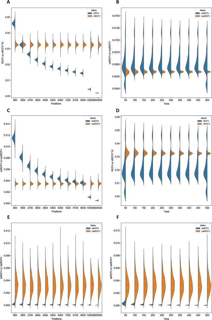
But this is also what RCFV did – nRCFV’s predecessor. What is unique about nRCFV is how it is normalized – the n of nRCFV. Basically, we found that RCFV gave higher values to smaller alignments: it said that smaller alignments were more likely to violate the stationarity assumption than big ones. This is due to a problem with the F of RCFV: Frequency. Frequencies are percentages. This means that the single change from an A to a T in a 100 nucleotide-long sequence is a 1% change in the composition of the sequence, but the same change in a 1000 nucleotide-long sequence is only a 0.1% change. So there needed to be some additional number crunching to balance that effect out, so that RCFV no longer penalized relatively small changes to small sequences.

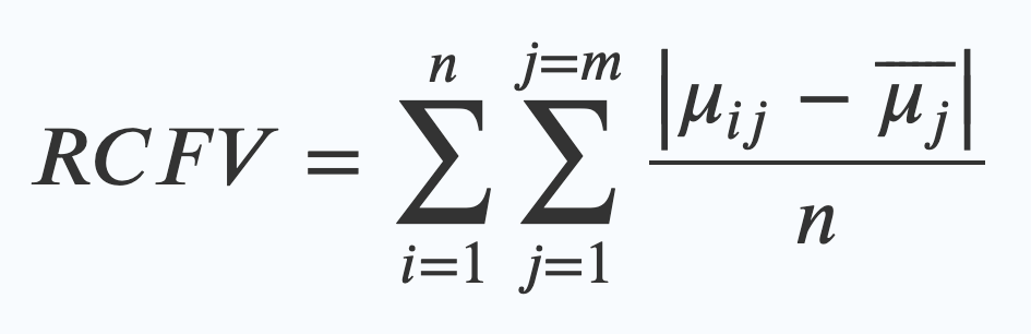
This is the original RCFV equation. The maths looks scary, but what it really means is quite simple. What it’s saying is that in order to work out the RCFV you have to:

1. Find the average frequency (a percentage expressed as 0-1, so 60% is 0.6) of one of your four nucleotides for a sequence in your dataset (that’s the μ_ij bit)
2. Work out the difference between that number and the average frequency of that same nucleotide across the whole dataset (that’s the μ_j wearing a hat). (These bars on the top | | mean you just measure the difference, so that 0.3-0.1 is the same as 0.1-0.3, just 0.2, rather than dealing with minus numbers)
3. Divide that number by how many taxa are in your alignment (that’s n)
4. Then repeat that for every nucleotide, and then every character and add all of those numbers together. (that’s what the Σ mean – the one on the right is the one that sums up the numbers for every character – j=m – and the one on the left sums up every taxa in the alignment – n)

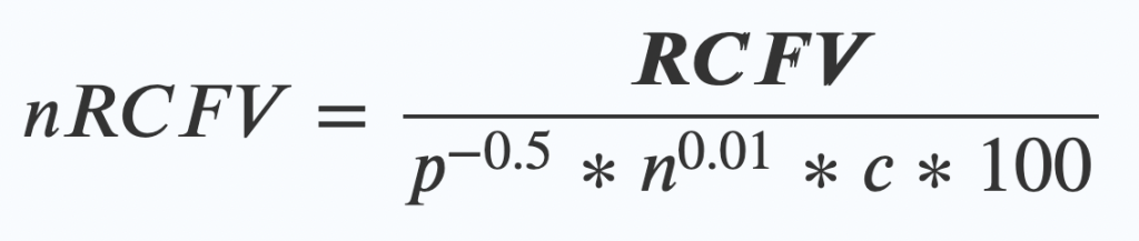
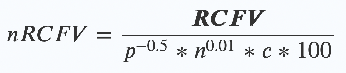
nRCFV adds one final step. Once you’ve worked out your RCFV value, then you apply this new “normalising constant” by dividing your RCFV by this bunch of friendly values:

1. The length of your alignment (p) to the power of -0.5.
2. Multiplied by….
   The number of taxa (n again!) in your alignment to the power of 0.01
3. Multiplied by….
   The number of possible things that character could have been (c) – so for a nucleotide dataset of ATCG, that means 4.
4. Multiplied by 100 (this last bit just makes the numbers look nice at the end)

We found that this can have some extreme effects! Some studies in the past have used RCFV to select data that was best to use for phylogenetic analysis (because it was thought to be data that didn’t violate the assumptions of our models). But when we took an example of this from 6 years ago and reselected the genes based on nRCFV rather than RCFV, we found that the top sixth of genes selected by nRCFV was 44% different to the top sixth selected by RCFV, because RCFV had eliminated many smaller genes from the running!

We’ve made nRCFV available for free for anyone to use through our github – that’s the standard practice for this kind of thing. Hopefully this will prove useful for many biologists in the future, and the assumption of Stationarity might not make as much of an ass out of you and me.